What is Factor Analysis?
Factor analysis is a multivariate analysis method used to explore and explain the structure of relationships between variables. It’s often applied in psychology and social science disciplines to identify the dimensions or factors that explain the relationships between variables. In this post, we will focus on how to conduct a factor analysis in SPSS and the methods available for extracting factors. We will also discuss how to interpret the results and what factors are important when assessing the quality of factor analysis.
Whenever data is collected, there’s the challenge of many variables correlating with each other. This situation can lead to issues in methods like regression, which is why multiple variables containing similar information are combined into factors (also called components). Variables that correlate strongly with each other are grouped into a single factor. The aim is to create a variable that contains as much of the same information from several variables as possible. The challenge lies in reducing the data as much as possible while losing as little information as possible. In SPSS, this method is known as dimension reduction.
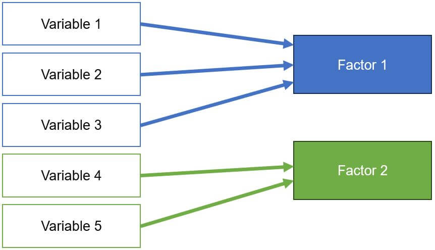
Factor analysis is a multivariate technique that calculates how strongly each variable loads on a theoretical factor. The stronger a variable’s loading, the higher its association with the theoretical factor, indicating shared similar information. This aggregation of variables (items) is purely mathematical. Ensure that the combination makes logical sense.
Where is the example data set?
You can find die data here
Prerequisites for Factor Analysis and Principal Component Analysis (PCA)
- Checking Linearity: Linearity should be present. A guide to checking linearity can be found here.
- Checking for Outliers: Outliers are values that are unusually small or large and can negatively impact the analysis by distorting results. The fewer outliers in a dataset, the better. A guide to checking statistical outliers is available here.
- Normal Distribution: The variables should be normally distributed. A guide for checking this is available here.
- Continuity: A continuous relationship between variables is assumed.
- Scale Level: Interval-scaled variables are necessary. Guide to scale levels.
- Number of Cases: Sample size. Ideally, 4 to 20 cases per calculated variable. A principal component analysis with 5 variables would require 20 to 100 subjects. As a rule of thumb, there should be 5 cases or 10 per variable, and anything under 100 total subjects should be critically evaluated.
Excursion: Explaining Rotation Methods
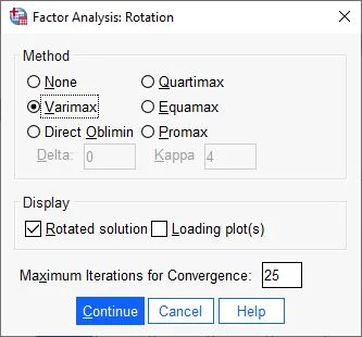
Varimax enhances the loadings, simplifying the assignment of variables. Large loadings are enlarged, and small loadings are reduced.
Quartimax: Similar to Varimax, but with a tendency for a variable to load more on one factor.
Equamax (or Equamax) is a compromise between Quartimax and Varimax. Factors are delineated while loadings are emphasized.
Promax is an oblique method: Initially, a Varimax rotation is performed, in which the factor loadings are further exponentiated. This amplifies large effects and diminishes smaller ones, simplifying interpretability.
Conducting Factor Analysis in SPSS
Calculating Principal Component Analysis in SPSS (Factor Analysis)
Menu Selection

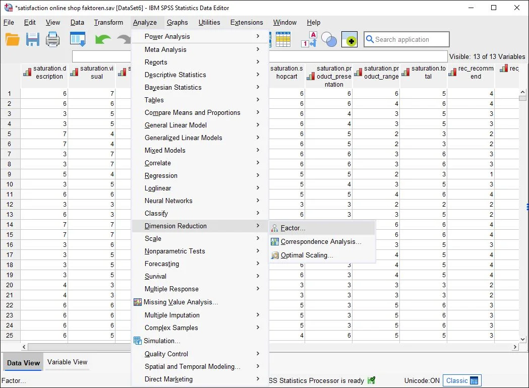
Step 1 in SPSS Factor Analysis and Principal Component Analysis: Menu Selection On the interface, click Analyze > Dimension Reduction > Factor Analysis…
Selecting Data

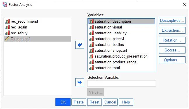
Step 2 in SPSS Factor Analysis and Principal Component Analysis: Assigning Variables In the dialog box, we see two columns. On the left, all available variables in the dataset are displayed. We select the variables for the principal component analysis and drag them to the right column (Variables).
Once all selected variables are in the right field, we start adjusting the principal component analysis.
Next, we click on the Descriptives button.
Selecting Descriptive Statistics for Factor Analysis

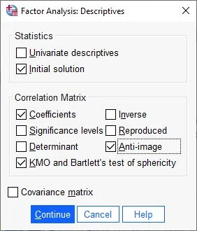
In the following dialog box, under Statistics, we choose Initial Solution. In the Correlation Matrix field, we check the boxes for Coefficients, Anti-Image, KMO, and Bartlett’s Test of Sphericity
We then confirm the entries by clicking Continue.
Selection of Extraction

Next, we choose Extraction on the right side of the dialog box.
Determining Extraction

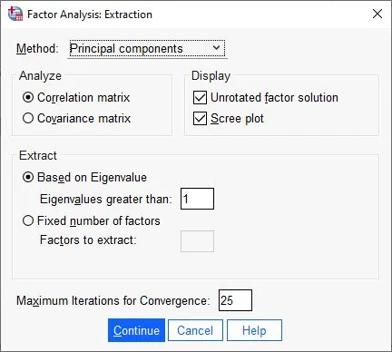
For methods, we choose Principal Components. In the Analyze field, we choose Correlation Matrix and under Display, select Unrotated Factor Solution and Scree Plot. All other settings should be as shown in the screenshot for this step.
We confirm the entries by clicking Continue.
Selection of Extraction

Next, we click on Rotation.
In the following dialog box, we choose a rotation method. The most common method is Varimax. In the Display field, we select the Rotated Solution button and click Continue.
Selecting Options

Next, we choose the Options button on the right side.
Determining Options for Principal Component Analysis

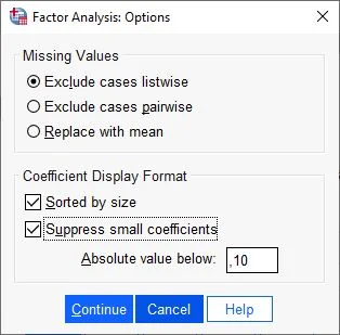
In the Coefficient Display Format section, we check the box for Sorted by Size, Suppress Small Coefficients. Absolute value under should be .10.
Then click Continue.
Ready to Start

That’s it for the settings. A click on OK starts the calculation of the principal component analysis.
Interpreting the Results of Principal Component Analysis
Correlation Tables
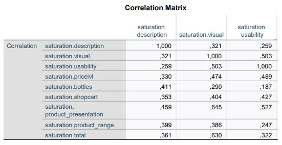
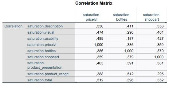
As comprehensive as the configuration of the principal component analysis was, the evaluations are just as extensive. First, we look at the correlation matrix table. This table shows us the correlations between the variables. Since the variables of a factor should correlate, we check here if there are variables that do not correlate with others (at least .30). Such variables should be removed to improve the overall analysis. Also, we do not want variables that correlate more than .90, as this could indicate multicollinearity.
KMO Criterion and Bartlett’s Test of Sphericity
One of the most important outputs is the Kaiser-Meyer-Olkin (KMO) Criterion. The KMO Criterion is the key criterion for determining the quality of the calculation. The value should never fall below the minimum of .50. The highest theoretical value is 1.00.
The second important criterion is Bartlett’s Test of Sphericity, which confirms a relationship between the variables. To proceed with the principal component analysis, the significance according to Bartlett must be significant, i.e., P-value of at least p<.05.

Summary
The KMO value should be at least .50, and the significance of Bartlett’s Test of Sphericity p=.05 or lower. If this is not the case, the calculation should be discontinued.
In our example, the KMO value is .83 and Bartlett’s Test of Sphericity is highly significant (p<.001). We can proceed with the principal component analysis.
Anti-Image Matrices
The KMO Criterion analyzes the relationship of all variables. The Anti-Image Matrices provide similar information for individual variables. Here too, all variables should have a value of at least .50, as indicated in the red-marked areas in the screenshot. In our example, all variables meet similar values to the KMO value (.83).
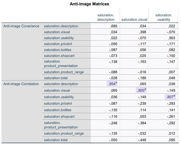
Table ‘Explained Total Variance’
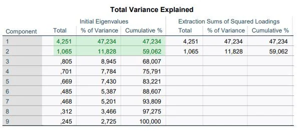
SPSS is generous in creating factors. It always creates as many factors as there are variables. Using this table, we decide to what extent the 9 variables can be summarized in a few factors.
We look at the column “initial eigenvalues (Initial Eigenvalues)” and there at “Total”. We only take factors that have eigenvalues of at least 1.00. Two components meet this criterion. That means the number of components can be set to two.
Furthermore, the table shows that the first factor can explain 47.23% of the total variance. Both factors together (cumulative %) explain 59.06% of the total variance, which indicates an information loss of 40%.
Determining the Number of Factors
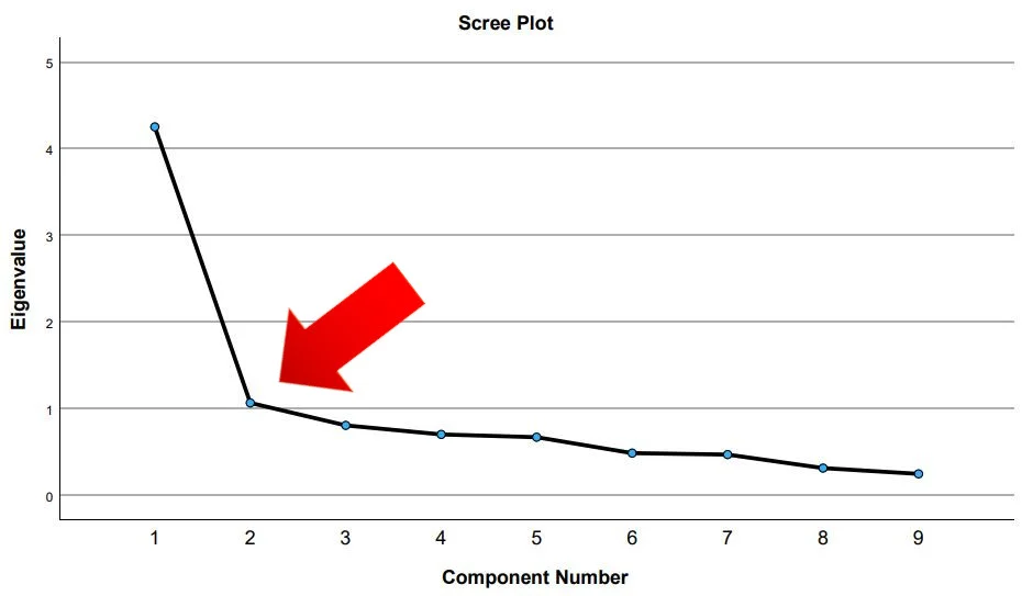
The number of factors can also be determined with a Scree Plot. The point where the so-called “elbow” sits indicates the number of factors. In our example, it’s 2.
Rotated Component Matrix
The rotated component matrix is the heart of the principal component analysis. The columns Component 1 and 2 show the respective loadings of each variable on one of the two components. The Varimax rotation has made the loadings clearer. They can range from 1 to -1. Some variables load on both components; in this case, we assign a variable to the strongest loading.
In our data analysis, the first six variables load on the first component. The last three variables load on factor 2.
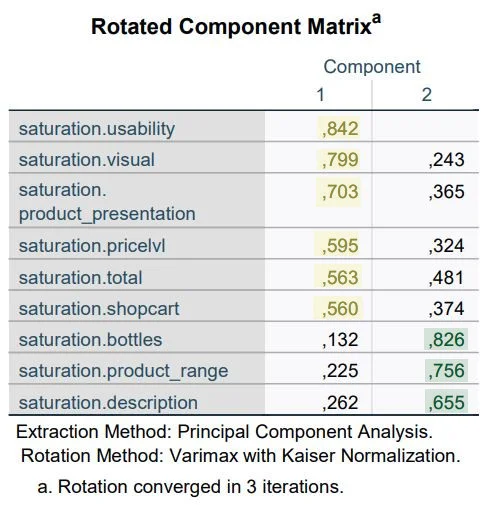
Note: Compare the rotated component matrix with the unrotated matrix to see the differences.
What Next?
Our analyses have shown that we can form two factors from our original 9 variables. This means that with two variables, we essentially have as much explanatory powerStatistische Power Statistische Power ist die Wahrscheinlichkeit, dass ein statistisches Testverfahren einen wirklich vorhandenen Unterschied zwischen zwei Gruppen oder Bedingungen erkennen wird. Eine hohe statistische Power bedeutet, dass das Testverfahren empfindlich genug ist, um kleine Unterschiede zu erkennen, während eine niedrige statistische Power dazu führen kann, dass wichtige Unterschiede übersehen werden. Es ist wichtig, dass die statistische Power bei der Planung einer Studie berücksichtigt wird, um sicherzustellen, dass das Testverfahren ausreichend empfindlich ist, um wichtige Unterschiede zu erkennen. as with 9 variables. The next step is to create these factors independently. Here, SPSS does not do the work for us. In the last part of this introduction, you will learn how to create the first dimension.
Creating New Variables
Menu Selection
In the menu, we select: Transform > Compute Variable

Calculating Variables in SPSS
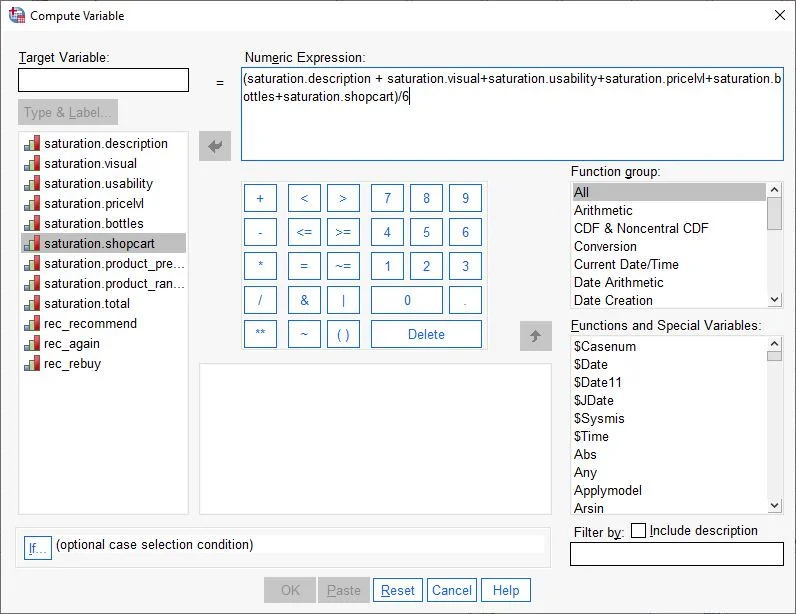
The “Compute Variable” dialog box opens.
First, in the Target Variable field at the top left, we enter the name of the new variable (e.g., Dimension 1). Then, we drag the first variable from the left column into the Numeric Expression field. Next, we press the plus sign (+) on the keyboard. We then drag the next variable of the first factor into the Numeric Expression field and press the plus sign again. We repeat this until we have all the variables of the factor as a sum in the field (see screenshot).
After all variables in the Numeric Expression field are understood as an addition, we enclose the total result in brackets. Then, we divide the total sum by the number of variables used in our equation. In our case, we use 6 variables, so we divide by 6. Our new factor should not be the sum, but the arithmetic mean of the included variables.
We confirm the entries and click OK.
New Variable in the Dataset
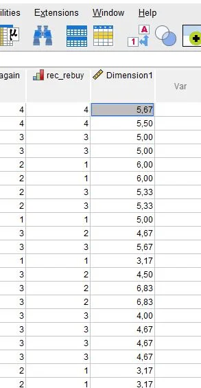
In the Data View, we see the new variable “Dimension1”, which summarizes the first six variables.
Further Steps
In our example, we have nine variables and have formed two factors. Both factors are an attempt to measure a theoretical construct regarding satisfaction with the online shop. A necessary prerequisite for this measurement instrument is reliability. Therefore, our next step should be a reliability analysis. Here is the guide to Reliability Analysis (Cronbach’s Alpha).
Conclusion on Principal Component Analysis in SPSS
Overall, factor analysis or principal component analysis is a powerful analytical tool used in many disciplines to explore and explain the structure of relationships between variables. It can serve both exploratory and confirmatory purposes, and there are various methods that can be used to extract factors. It’s important to assess the quality of the factor analysis and ensure that it is valid and reliable before interpreting the results and applying them to the data. When applied carefully and critically, factor analysis can be a useful tool to understand and explain the structure of relationships between variables.
5 Facts About Factor Analysis in SPSS
- Factor analysis is a multivariate analysis method used to explore the structure of relationships between variables. It aims to investigate and explain cause-and-effect relationships between variables.
- Factor analysis is often applied in psychology and social science disciplines to identify the dimensions or factors that explain the relationships between variables.
- Factor analysis can serve both exploratory and confirmatory purposes. Exploratory factor analysis is used to discover new structures or factors, while confirmatory factor analysis confirms known structures or factors.
- In factor analysis, relationships between variables are modeled using eigenvectors and eigenvalues. Eigenvectors are vectors that describe the structure of relationships between variables, while eigenvalues indicate the strength of these relationships.
- Factor analysis is a flexible analytical tool, and there are various methods that can be used to extract factors, including principal component analysis and Varimax rotation. The choice of the appropriate method depends on the objectives and characteristics of the data.
Frequently Asked Questions and Answers: Principal Component Analysis and Factor Analysis in SPSS
What is the Goal of Factor Analysis?
The goal of factor analysis is to summarize a large number of variables into fewer variables that describe the key characteristics of the data. These summarized variables, known as factors, can be used to understand the structure of the data and make predictions about it. Factor analysis is employed to reduce and understand the dimensions or characteristics of the data, and how the variables are interrelated. It’s also used to eliminate redundant information and simplify the analysis of data with many variables. Overall, the aim of factor analysis is to recognize and understand the structure of the data by identifying and summarizing its key characteristics. It’s widely used in areas such as psychology, marketing research, and social sciences.
How Does Factor Analysis (Principal Component Analysis) Work?
Factor analysis is a statistical method used to summarize a large number of variables into fewer variables, known as factors.
The factor analysis process involves several steps:
– Preprocessing: Ensuring the data is suitable for analysis, including completeness, consistency, and the absence of outliers or erroneous values.
– Factor Identification: Calculating correlations between variables to create a correlation matrix, then using a factor method to identify factors that best describe these correlations. Methods like principal component analysis or rotation methods can be used.
– Factor Estimation: Once factors are identified, factor values for each case are calculated, which can be used for predictions about the data.
– Factor Interpretation: Interpreting the factors to understand what they mean and how they influence the variables. It’s also crucial to verify the reliability and validity of the factors.
Overall, factor analysis is a useful method for reducing the complexity of data with many variables and identifying key features of the data. It’s frequently used in psychology, marketing research, and social sciences.
When is Principal Component Analysis (PCA) Useful?
Principal Component Analysis (PCA) is a statistical method used to summarize a large number of variables into fewer variables known as principal components.
PCA is valuable when trying to understand and reduce the structure of data with many variables. It’s used for reducing and understanding the dimensions or characteristics of the data, how the variables relate to each other, and for eliminating redundant information to simplify data analysis with many variables.
What Questions Are Addressed with Factor Analyses?
Factor analyses are used in many areas where the goal is to understand and reduce the structure of data with many variables. They are applied in various fields, including:
– Psychology: To investigate dimensions of personality traits or other psychological constructs.
– Marketing Research: To understand customer survey structures and identify factors that best describe customer attitudes and behaviors.
– Social Sciences: To understand the structure of social phenomena and make predictions about social outcomes.
How Many Items Per Factor?
There is no fixed rule for how many items should be included per factor in a factor analysis. The number of items per factor depends on the specific characteristics of the data and the research question. Generally, each factor should contain at least three to four items to ensure adequate estimation of factor values. Fewer items per factor might result in less reliable factor value estimates. However, there’s no upper limit to the number of items per factor. In some cases, more items per factor may be beneficial for better estimation. The specific characteristics of the data and the research question should be considered when deciding how many items to include per factor in the analysis.
What is an Eigenvalue in Factor Analysis?
An eigenvalue is a measure of the variability explained by a factor in factor analysis. A high eigenvalue indicates that the factor explains a significant portion of the data’s variability, whereas a low eigenvalue means it explains only a minor part. In factor analysis, eigenvalues are used to assess the importance of the factors. A factor with a high eigenvalue is generally considered more important than one with a low eigenvalue, as it explains a greater proportion of the data’s variability. It’s important to note that eigenvalues cannot be directly compared as they are measured in different units. Instead, eigenvalues are usually represented as percentages of the variability explained by each factor, known as eigenvalue decomposition, and are used to assess the importance of the factors concerning the overall variability of the data.
What is Exploratory Factor Analysis?
Exploratory factor analysis is a type of factor analysis used to investigate and understand the structure of data. Unlike confirmatory factor analysis, which aims to test a pre-formulated model of the data’s structure, the goal of exploratory factor analysis is to discover and explore the data’s structure. In exploratory factor analysis, correlations between variables are calculated, and a correlation matrix is created. Then, a factor method is used to identify the factors that best describe these correlations. Various factor methods can be applied, such as principal component analysis or rotation methods. After identifying the factors, factor

