What is multiple linear regression?
Multiple linear regression is a technique for modeling the relationship between a dependent variable (also called the target variable) and multiple independent variables (also called predictors). Multiple linear regression is used to estimate a linear relationship between variables and predict how the dependent variable will change based on changes in the independent variables.
An example of using multiple linear regression might be to predict the effect of age, gender, and education level on a person’s income. In this case, income would be the dependent variable and age, gender, and education level would be the independent variables.
What does a multiple linear regression calculate?
A multiple linear regression calculates coefficients for each of the independent variables (also called predictors) that indicate how much the dependent variable (also called the target variable) will change with a unit change in the independent variable if all other variables remain constant.
The coefficients are calculated by minimizing the sum of squared errors (also called residuals) between the actual values of the dependent variable and the predicted values obtained from estimating the coefficients.
Multiple linear regression also provides a prediction for the dependent variable based on the specified values of the independent variable. This prediction can be used to determine how the dependent variable will change under different conditions.
It is important to note that multiple linear regression is only valid if the assumptions of linear regression are met, such as linear relationship between the variables and normal distribution of the residuals.
Multiple linear regression in the manual
In statistics, we often try to explain the influence of one variable on another: Does the value of a used car depend on the age of the car? The problem with such an isolated view is that in reality, several influences can act simultaneously. The value of a used car could depend on its age, but also on the kilometers driven – or the number of accidents. Theoretically, there are any number of influencing factors that can exert an influence to varying degrees.

In order to be able to examine a more precise statement about the influences of variables (predictors) on a target variable (criterion), multiple linear regression analysis is therefore used in statistics. It extends the simple linear regression with additional predictors. In our example, the value of the used car is the target variable and several predictors can be considered as predictors: the mileage, the age, engine powerStatistische Power Statistische Power ist die Wahrscheinlichkeit, dass ein statistisches Testverfahren einen wirklich vorhandenen Unterschied zwischen zwei Gruppen oder Bedingungen erkennen wird. Eine hohe statistische Power bedeutet, dass das Testverfahren empfindlich genug ist, um kleine Unterschiede zu erkennen, während eine niedrige statistische Power dazu führen kann, dass wichtige Unterschiede übersehen werden. Es ist wichtig, dass die statistische Power bei der Planung einer Studie berücksichtigt wird, um sicherzustellen, dass das Testverfahren ausreichend empfindlich ist, um wichtige Unterschiede zu erkennen. (HP), fuel consumption, car brand and equipment characteristics such as fuel (gasoline/diesel/electric), emission class and so on.
With multiple linear regression, statisticians try to understand which predictors exert a significant influence on the criterion. We want to find out how strong the influence is and which variables are less important to calculate a correlation. The goal is to create a mathematical equation (predictive model) that can predict the value of a used car as accurately as possible with data such as age and mileage. How this equation can look like and how the precision of the equation (variance elucidation) is measured is explained step by step in this tutorial at the end.
Where can I find the sample data set for the calculation in SPSS?
The sample data set is here.
Results can be produced relatively quickly thanks to SPSS. The difference between a good and a bad analysis is to check if certain arithmetic operations may be feasible at all and what might affect the precision of the results.
- Level of measurement: The target variable (criterion) must be a dependent variable and interval scaled (what does that mean?). The predictors must be at least two independent variables. The predictors can be either nominally scaled or at least interval scaled. Learn more about Level of measurement.
- Linearity: In a multiple linear regression analysis, the variables under study must have a linear relationship. If this is not the case, there may be underestimation or overestimation in the predictive model. Check linear relationship guide.
- Outliers: Multiple linear regression is sensitive to outliers, so the data set should be checked for outliers. Instructions Checking for Outliers.
There are other conditions for multiple linear regression that we need to consider. These are best analyzed once we have done the initial calculations in SPSS. And this is exactly what happens in the next step.
Es gibt weitere Voraussetzungen für eine multiple lineare Regression, die wir beachten müssen. Diese lassen sich am besten analysieren, wenn wir die ersten Berechnungen in SPSS durchgeführt haben. Und genau das passiert im nächsten Schritt.
Perform multiple linear regression in SPSS
Perform Multiple Linear Regression calculation in SPSS.
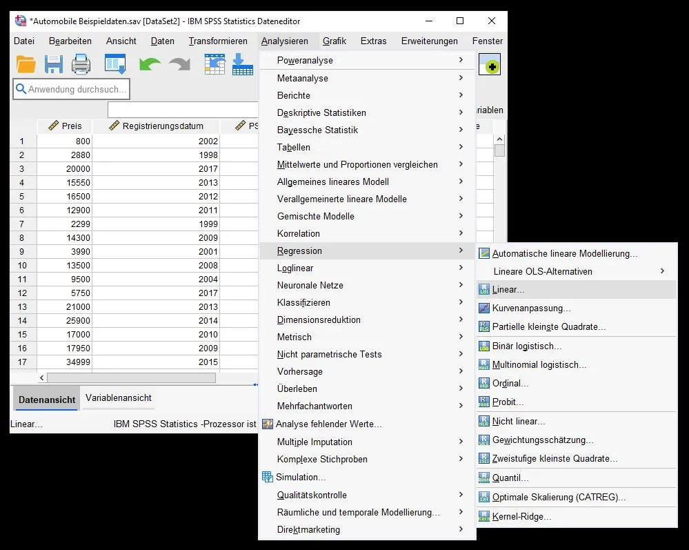
Select Multiple Linear Regression in SPSS

To run a multiple linear regression, we go to Analyze > Regression > Linear…
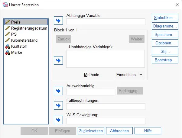
Dialog box: Linear Regression

The Linear Regression dialog box opens. A dialog box is a window that has been opened by the system and is waiting for your input.
On the left side we see our available variables from the dataset. On the right side we see several fields where we can move variables. There are two ways to move the variables:
Drag-and-drop: we click on a variable with the left mouse button, hold the mouse button down and drag it to the desired field, then release the mouse button.
Using the button: we select a variable with the left mouse button and click again with the left mouse button on the arrow that points to the right and is located next to the right fields.
Assign variables in SPSS

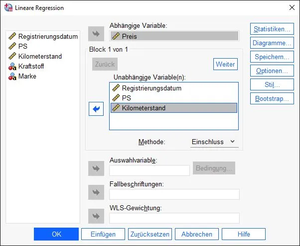
Now we put the regression together. For this we need a dependent variable. The goal of multiple linear regression is to explain the variance of the values of a dependent variable by multiple independent variables.
For our example, we want to explain the price of a used car by characteristics such as horsepower, mileage, and registration date.Therefore, price is the independent variable. The other variables go into the “independent variable(s)” field.
Perform other settings

We are still in the same dialog box. Before we start the calculations, SPSS allows us to make settings. These settings are located on the right side of the dialog box behind several buttons.
We click on the “Statistics” option on the right side of the dialog box.
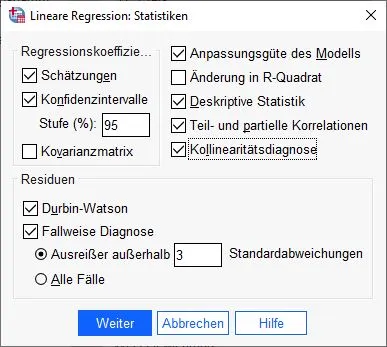
Linear Regression: Configure Statistics

At first glance, the settings look confusing. This is because SPSS knows many calculations. We need certain statistics to analyze our results in more detail and to check preconditions. For this reason we select the following options:
Estimates, Confidence Intervals (95%), Goodness of Fit of Model, Descriptive Statistics, Partial and Partial Correlations, Collinearity Diagnosis, Durbin-Watson, and Case-by-Case Diagnosis (3).
We have a lot to look forward to! We click Next to confirm the selection.
Perform other settings

We land back on the dialog box and select further settings. In the next step we click on “Diagrams” on the right side.
Multiple linear regression: Set charts

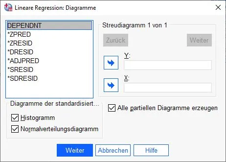
The next dialog box for diagrams appears. In the lower area we click on the check boxes Histogram, Normal distribution diagram and Generate all partial diagrams.
We confirm the entries and click the Next button.
Perform other settings

Back to the original dialog box. Here we click on the “Save” setting to create new variables.
Dialog box linear regression: Save
In this dialog box we select the following check boxes:
Predicted values: not standardized.
Residuals: Studentized
Residuals: Studentized, excluded
Distances: Cook and leverage values
Save covariance matrix
We confirm by clicking Next.Ready to go: we can start the calculation in SPSS

Done. We are ready to go and click OK to let SPSS calculate the multiple linear regression.
The analysis of the results follows in the next step.
Checking further prerequisites of the multiple linear regression
Before we jump into the results, we check further prerequisites for the regression in SPSS. We can see the necessary data in the new tables we created in the last step. They are all in the output.
Precondition: Independence of the residuals
When we analyze data, we assume that the sample under study was tested absolutely randomly. This means that the selection of and all elements and their combination does not follow any scheme. If this is not the case, our final model loses significance (autocorrelation). In SPSS we test the first order autocorrelation and clarify whether a residual correlates with its direct neighbor. Especially for tests with time series analyses, a test of autocorrelation is important.
What is a residual?
In statistics, the term “residual” refers to the deviation between the observed value and the predicted value in a regression model. Thus, it is the difference between the variable actually observed and the variable predicted by the model. The plural of residual is residuals.
Residuals are important in assessing the quality of a regression model. A good model will usually have small residuals, which means that the predictions of the model are very accurate. On the other hand, large residuals are considered an indication that the model is not well fitted and may need improvement.
Durbon-Watson statistics
We check the independence of the residuals in SPSS with the Durban-Watson statistic. In the instructions above, we put a check mark there for statistics in step 5. The table with the data is in the output and is called “Model Summary”.

We consider the column on the far right called “Durbin-Watson statistics”. An autocorrelation basically exists if …
- the value is higher than 2
- the value is lower than -2
If we obtain a value between 2 and -2 in the test, we can assume that no autocorrelation occurs. The Durbin-Watson statistic can theoretically take a value from 4 to -4.
In our example, we see a value of 1.622. An autocorrelation does not occur according to Durbin-Watson statistics.
What to do if there is an autocorrelation?
If there is an autocorrelation, another procedure should be used, such as heteroskedasticity-and-autocorrelation-consistent estimators (Newey-West estimators or HAC).
Precondition: No multicollinearity
If two or more variables have a very high correlation, we can assume that they contain similar “information” and the calculation of the regression coefficients will be affected. Therefore, our final model should use predictors that are not too similar (multicollinearity).
Testing multicollinearity using correlation tables.
A relatively simple way to measure multicollinearity is to test correlations. Therefore, in this issue we look at the correlations table.
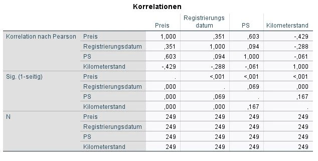
In this table we look at the top rows that belong to “Pearson’s correlation”: Price, Registration Date, Horsepower and Mileage. These variables are in the columns and rows. This means that we want to quickly compare the correlations between each variable.
The values for correlations can range from 1 to -1. A 1 means a perfect correlation. -1 is a perfect negative correlation and 0 means no correlation.
Briefly explained: What is a correlation?
In statistics, the term “correlation” refers to the extent to which two variables are related. When two variables are correlated, it means that they are related in some way and that a change in one variable is likely to cause a change in the other variable. There are different types of correlation, such as positive, negative, and no correlation.
A positive correlation means that if one variable increases, the other variable will also increase. A negative correlation means that when one variable increases, the other variable decreases. No correlation means that there is no relationship between the two variables.
It is important to note that correlation is not the same as causation. That is, just because two variables are correlated does not necessarily mean that one variable directly affects the other. There may be other factors that influence the relationship between the variables.
An example of a positive correlation would be the relationship between age and experience. In this case, one might assume that the older someone is, the more experience he or she tends to have. So, if we consider age as the dependent variable and experience as the independent variable, then the correlation between these two variables would be positive. That is, as age increases, experience is likely to increase and vice versa.
An example of a negative correlation would be the relationship between body weight and exercise. In this case, one might suspect that the more someone exercises, the less likely he or she is to be overweight. So, if we consider the amount of exercise as the dependent variable and body weight as the independent variable, the correlation between these two variables would be negative. That is, as body weight increases, the amount of exercise likely decreases and vice versa.
However, it is important to note that this is only a guess and there could be other factors that influence the relationship between these two variables. To ensure that there is indeed a negative correlation, one would need to analyze the data to determine the strength and direction of the relationship.
As soon as two variables have a correlation of 0.7 or higher, we can assume multicollinearity. This is also true for negative values of -0.7 and smaller.
In our example, there are correlations of 0.351, 0.603, -0.429, and so on. We can therefore rule out multicollinearity.
Testing multicollinearity by tolerance and VIF
Another method is the test by tolerance and VIF in the table coefficients (VIF stands for variance influence factor).

We look at the far right of the “Tolerance” and “VIF” collinearity statistics columns. Multicollinearity is present if one of the two conditions is met:
- the VIF value is above 10
- the tolerance value is below 0.1
In our example, this does not apply to any of the variables (horsepower, mileage, registration date). We can exclude multicollinearity.
Was tun, wenn es eine Multikollinearität gibt?
If multicollinearity is found, then there are variables that are too similar. Here you should ask yourself if it makes sense to use two variables that basically say the same thing. For this reason, it may make sense to remove one variable. If you have two or more predictors, this is the easiest solution.
Multicollinearity is an indicator that your data set has variables that are too similar. Statistical experts like to apply principal component analysis (factor analysis) in this case. Using this method, we can create one variable from several variables and condense information. Here is the tutorial on principal component analysis.
Prerequisite: Homoscedasticity of the residuals
At best, the variance of the residuals should be equal, so that in the later equation certain areas (high-priced cars, low-priced cars) do not have different precision statements. At best, our final model should be able to calculate accurate results in all areas.
To check the homoscedasticity of the residuals in SPSS, we recommend this guide.
Prerequisite: Normal distribution of residuals
Residuals must be normally distributed, homoscedastic, and independent. This is important for the validation of the results, so the reliability of the results is ensured.
Histogram of the residuals as a method of analysis
This histogram shows the frequency and the distribution of the residuals for the variable price.
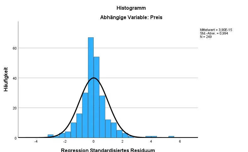
In our example, the residuals for the variable price lie quite clearly on the course of the normal distribution, which is good. At the top right we see the mean, standard deviation and number of cases (N). The mean should ideally be around 0 and the standard deviation around 1. The number of cases should also be sufficiently high.
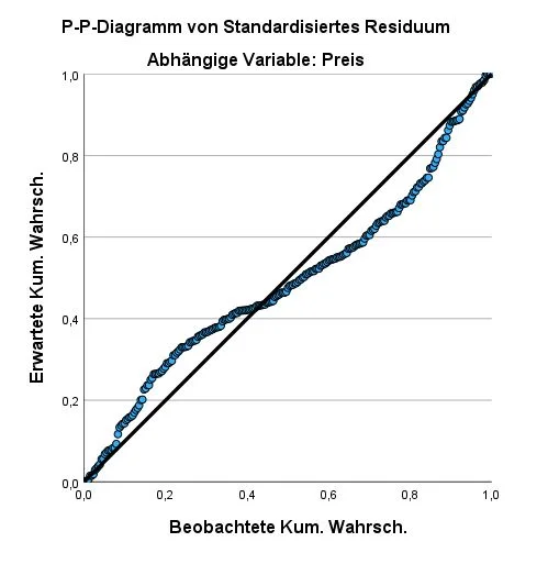
Method: P-P plot diagram
This P-P plot shows that the observable values (circles) are quite close to the expected values (line). It is not perfect, but still acceptable. The closer the observable values are to the line, the better. If the observable values are quite far away, it speaks against a normal distribution.
Method: Shapiro-Wilk test
The normal distribution can take place by means of Shapiro-Wilk test with the variable SRE_1.
Here are the instructions for the Shapiro-Wilk test.
What happens if the normal distribution is not given?
- You simply continue the calculation and refer to it in the results. Usually, multiple linear regression is quite robust against violation and your results are still usable.
- Alternatively, your data can be transformed. The problem with transforming is that it can lead to aggravation, which is also problematic in statistics.
- Alternatively, you can use bootstrappingBootstrapping Bootstrapping ist eine Methode der Datenanalyse, bei der aus einer bestehenden Stichprobe wiederholt neue Stichproben gezogen werden, um die Unsicherheit von Schätzungen und die Stabilität von Statistiken zu untersuchen. Durch das Bootstrapping wird die Verteilung der Schätzungen simuliert und es können Konfidenzintervalle berechnet werden, die eine Aussage über die Wahrscheinlichkeit machen, dass die wahre Population innerhalb eines bestimmten Bereichs liegt. in SPSS. This option is available in the settings of a multiple linear regression.
- Other regression methods such as Constrained Nonlinear Regression (CNLR) can be performed. It is much more robust, but also more complex to perform.
Analysis of the results
Analysis of the variance explanation of our regression model
We look at the Model Summary table and there the columns R, R² and corrected R².

- R is the Pearson correlation coefficient, which measures the strength and direction of a linear relationship between two variables. R is always between -1 and 1, where -1 indicates a perfect negative correlation, 1 indicates a perfect positive correlation, and 0 indicates no correlation.
- R² is the variance explanation and indicates how much of the variation in the dependent variable is explained by the independent variable. R² is always between 0 and 1, where 1 means that the independent variable explains all of the variation in the dependent variable and 0 means that the independent variable offers no explanation for the variation in the dependent variable.
- Corrected R² is an adjusted version of R² that takes into account how many variables were analyzed in the regression. It is used to compare how well different regression models explain the dependent variable and indicates how much of the variation in the dependent variable is explained by the independent variables when the number of variables is taken into account. Like R², corrected R² is always between 0 and 1.
Cohen gives us an interpretive aid:
| |R| | |R²| und korrigiertes |R²| | Interpretation according to Cohen |
|---|---|---|
| .10 | .02 | Weak correlation |
| .30 | .13 | Moderate correlation |
| .50 | .26 | Strong correlation |
Don’t forget that these are only guidelines and the interpretation is often quite more complex. For example, in neuroscience studies, smaller R can be a strong result because the sensory system may have certain limitations. It is often a good idea to look at similar studies by other researchers. This will give you a better sense of what your expectations should be.
In our example, R² has the value of .555 and a corrected R² of .550, which is an excellent result.
Analysis of the significance of the model
We look at the ANOVA table and there at the rightmost column: Significance (Sig.).

We asked ourselves whether our result was purely random or whether there was a significant correlation. In statistics, significance is denoted by the variable “p”. The smaller the p-value, the higher the significance. The significance cannot theoretically add up to zero, which is why SPSS gives us a p <.001 for very small values. In our example, the result is highly significant.Whether the results in your study are significant or not depends on the significance level used. The significance level is abbreviated with the Greek letter “α” and is usually α= .05. A significance level of 5% means that we accept the result of the model with a probability of error of 5%.
What should the significance level be?
The significance level is the threshold that determines how likely it must be that an outcome occurs due to chance before it is assumed to occur due to an actual relationship between two variables. It is usually specified as an alpha value and is usually set at 0.05 or 0.01. A lower significance level means having more stringent requirements before assuming that a result is significant, while a higher significance level means having less stringent requirements. Choosing the right significance level depends on the objectives of the study and the risks one is willing to take of being false negative or false positive.
Die Regressionsgleichung
The regression equation
The regression equation is the heart of our model. It is the mathematical formula to predict values for our target variable.
What does the regression equation mean?
In regression analysis, a regression equation is used to describe the relationship between a dependent variable and one or more independent variables. In general form, the regression equation looks like this:
y = b0 + b1 * x1 + b2 * x2 + ... + bn * xnIn this equation, y is the dependent variable, the predictor variable or the one to be explained, and x1, x2, …, xn are the independent variables or the predictors used to explain y. b0 is the y-intercept and b1, b2, …, bn are the regression coefficients (also called slope coefficients) for the independent variables. The regression coefficients indicate how much y changes when one independent variable changes by 1 while all other variables remain constant.
The regression equation is used to make predictions for y by substituting the known values for the independent variables
Analyze coefficients table
We look at the Coefficients table in SPSS and there at the column “Regression Coefficients B”. In each row here we see the values for our dependent variables: Registration date, horsepower and mileage, and the constant.

For example, if you want to know how the number of miles driven affects the value of a used car. In this case, one could use a regression equation to describe the relationship between these two variables. The regression equation is used to calculate predictions for the average price on a used car.
Our equation can do even more: if we enter the registration date, the horsepower number and the mileage, we can quite accurately determine the price of a used car. We just need to use the formula below:
Preis = 220,998 * Registrierungsdatum + 89,952 * PS - 0,069 * Kilometerstand – 439666,563
Konkret sagt uns unsere Gleichung
- The higher the registration date, the higher is price. For each year the price increases by 220.998 USD.
- The higher the horsepower number, the higher the price. For each horsepower more the price increases by 89,952 USD.
- The lower the mileage, the higher the price. For each kilometer driven, the price decreases by 0.069 USD.
How can I calculate the price with the equation?
7115,10 = 220998 * 2010 + 89952 * 90 - 0,069 * 80000 - 439666,563We test our regression equation. Suppose I have a used car with registration date 2010 , with 90 hp and 80,000 kilometers driven, then the value of the used car is 7,115.10 EUR.
This model has a generality. We can enter any values and get a predicted value.
Checking the significance values
In the next step we check the significance of the coefficients. In the Coefficients table, we therefore look at the “Sig.” column and see the p-values.
In our example, all predictors are significant.
My model is significant, individual coefficients are not. What to do?
This may be due to multicollinearity, which we reported above. Another reason is having too many predictors in the equation. If there are too many predictors or cases, the significance test can be biased. In this case, you should exclude the non-significant variable and recalculate the model.
Calculate effect sizes
Um die Effektstärken zu berechnen, gibt es einen hervorragenden Rechner auf statistikguru.de
Publish results
Eine AutokorrelationAutokorrelation Autokorrelation ist ein Maß für den Zusammenhang zwischen den Werten einer Variablen über Zeit oder anderen Dimensionen hinweg und kann verwendet werden, um zu bestimmen, ob es in den Daten Muster oder Trends gibt. Eine hohe Autokorrelation bedeutet, dass die Werte der Variablen in der Regel in die gleiche Richtung gehen, während eine niedrige Autokorrelation darauf hinweist, dass die Werte der Variablen zufällig verteilt sind. in den ResiduenResiduen Residuen sind die Abweichungen zwischen den beobachteten Daten und den durch ein statistisches Modell vorhergesagten Daten und werden verwendet, um die Anpassung des Modells an die Daten zu beurteilen und um mögliche Muster oder Trends in den Daten zu erkennen. Sie können auch verwendet werden, um die Validität und Zuverlässigkeit von Vorhersagemodellen zu überprüfen. lag nicht vor, da die Durbin-Watson-Statistik einen Wert von 1.622 aufweist.
Das Regressionsmodell zeigt einen R² = 0.555 (korrigertes R² = 0.550) und ist signifikant p<0.001 (α ≤ 0.5).
Die Prädiktoren Kilometerstand, PS und Registrierungsdatum sagen statistisch signifikant das Kriterium Preis eines Gebrauchtwagens voraus. Die Regressionsgleichung lautet Preis = 221.00 * Registrierungsdatum + 89.95 * PS + 0.07 * Kilometerstand – 439,666.56.
Tip when publishing
It often happens that not only one regression equation is calculated and several hypotheses are tested. In this case it can be useful to present the data as a table. Each additional equation is placed in a new row.
| Hypothesis | Regression | R² | Adj. R² | Sig. | DWS |
|---|---|---|---|---|---|
| H1 | Preis = 221.00 * Registrierungsdatum + 89.95 * PS + 0.07 * Kilometerstand – 439,666.56. | .555 | .550 | .001*** | 1.622 |
=p ≤ .05, ** = p ≤ .01, *** = p ≤ .001.
Frequently Asked Questions and Answers: Multiple Linear Regression
When is multiple linear regression used?
EMultiple linear regression is used when estimating the influence of multiple independent variables on a dependent variable and predicting how the dependent variable will change based on changes in the independent variables.
Multiple linear regression is a powerful analytical tool used in many areas of science, business, and other fields, for example, to study how age, gender, and education level affect a person’s income, or to determine how various marketing factors affect the sale of a product.
It is important to note that multiple linear regression is only valid if the assumptions of linear regression are met, such as linear relationship between variables and normal distribution of residuals. If these assumptions are not met, other methods of analysis such as nonlinear regression or multivariate regression may be considered.
What is the difference between linear and multiple regression?
The difference between linear regression and multiple regression is that linear regression uses only one independent variable (also called the predictor) to estimate the impact on the dependent variable (also called the target variable), while multiple regression uses multiple independent variables.
In linear regression, a linear relationship is estimated between the dependent variable and the independent variable, while in multiple regression, a linear relationship is estimated between the dependent variable and each of the independent variables.
Linear regression is a powerful analysis tool in many cases, but there are instances where multiple variables need to be considered to gain a more comprehensive understanding of the relationships between variables. In such cases, multiple regression may be an appropriate method of analysis.
It is important to note that multiple regression is only valid if the assumptions of linear regression are met, such as linear relationship between variables and normal distribution of residuals. If these assumptions are not met, other methods of analysis such as nonlinear regression or multivariate regression may be considered.
What are the types of regressions?
There are different types of regressions used depending on the nature of the dependent and independent variables and the form of the relationship between them. Here are some examples of different types of regressions:
– Linear regression: linear regression is used to describe the linear relationship between a dependent variable and an independent variable. The model consists of a straight regression line that represents the relationship between the variables.
– Multiple Linear Regression: Multiple linear regression is used when there are multiple independent variables to explain the dependent variable.
– Polynomial Regression: Polynomial regression is used when the relationship between the variables can be described by a curve rather than a straight line.
– Logistic Regression: Logistic regression is used when the dependent variable is binary, that is, it can take only two possible values (e.g., “yes” or “no”). It is often used to make predictions about the probability of events.
There are other regressions such as multinomial regression, which we will not discuss further here.
What does R2 mean in regressions?
The R2 (also known as “R²”, “coefficient of determination coefficient”) is a measure of how well a regression model explains the variability of the dependent variable. It is calculated by dividing the proportion of the variance of the dependent variable explained by the regression model by the total variance of the dependent variable.
The R2 takes values between 0 and 1, with a higher value meaning that the regression model provides a better explanation of the variability of the dependent variable. An R2 value of 0 means that the regression model provides no explanation of the variability of the dependent variable, while an R2 value of 1 means that the regression model fully explains the variability of the dependent variable.
It is important to note that R2 is not always a reliable measure of the predictive accuracy of a regression model, especially when the model is tested on new data.
More resources for multiple linear regression
How many observations are needed for a regression?
There is no hard and fast rule on how many observations one needs for a regression. The number of observations needed depends on several factors, such as the number of independent variables, the complexity of the regression model, and the strength of the relationship between the variables.
However, as a general rule, one should have enough observations to obtain a representative sample of the data and to ensure that the model fits the data sufficiently well. As a general rule, one should have at least 10 observations for each independent variable one introduces into the model. However, if the model is very complex or if the relationship between the variables is very weak, more observations might be needed.
It is important to note that one should not always have as many observations as possible. In some cases, it might make more sense to have fewer observations, but to choose them carefully to ensure that they are relevant and representative of the population to which you are referring.

