Descriptive analysis is a vital part of statistics, serving to summarize and describe data. With descriptive statistics, we can identify characteristic features of a sample or a population and infer conclusions about the underlying distribution. In this article, we will focus on descriptive analysis in SPSS, learning how to calculate and interpret various descriptive statistics using this program.
Descriptive analyses of frequencies are a great starting point to gain an overview of a dataset. In our example for this guide, we look at the market value of approximately 250 cars and analyze the distribution of prices, brands, and registration dates.
You can download the sample dataset here.
Descriptive Statistics in SPSS
Selecting Statistics and Charts

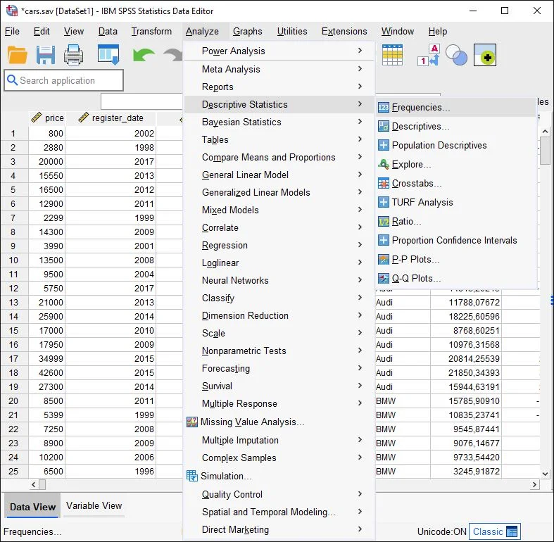
Step 1 in Descriptive Frequencies in SPSS: Menu Selection in SPSS Click on Analyze > Descriptive Statistics > Frequencies
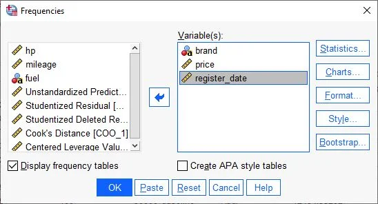
Frequencies Dialog Box

A dialog box with multiple fields appears. The left field is the variable list, displaying all available variables. To let SPSS know which variables to analyze, we drag our selection to the right field named “Variable(s)”. We either drag the individual variables into the right field or click once on the variable name and then click on the middle arrow between the fields, pointing right.
In our example, we select the variables Price, Registration Date, and Date. A check should be placed at the bottom option for showing frequency tables.
Next, we click on the Statistics button.
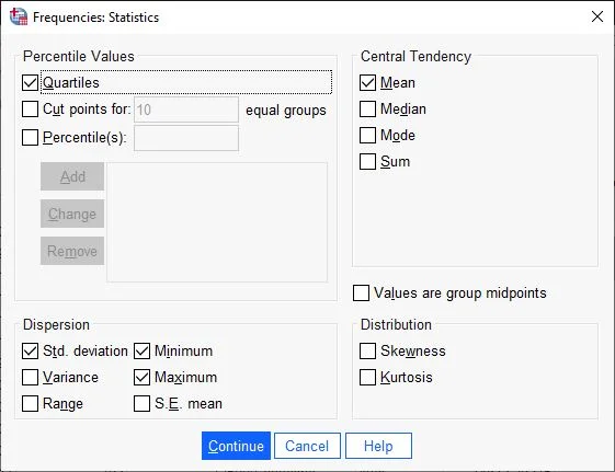
Statistics Dialog Box

Step 3 in Descriptive Frequencies in SPSS: Selecting Statistics, Quartiles, Mean, Standard Deviation, Minimum, Maximum A dialog box opens with a selection of statistical measures for frequency analyses. In our case, we choose the Mean option as a measure of central tendency (arithmetic mean) and in the Dispersion field, we select options for Standard Deviation (Std. deviationStandardabweichung Die Standardabweichung ist ein Maß für die Streuung der Werte einer Variablen um ihren Mittelwert und gibt an, wie sehr die Werte von ihrem Durchschnitt abweichen. Sie wird häufig verwendet, um die Varianz innerhalb einer Population oder Stichprobe zu beschreiben und kann verwendet werden, um die Normverteilung einer Variablen zu beschreiben. Eine kleine Standardabweichung bedeutet, dass die Werte der Variablen dicht um ihren Mittelwert clustern, während eine große Standardabweichung darauf hinweist, dass die Werte der Variablen weiter verteilt sind. ), Minimum, and Maximum. In the Percentile Values field, we check Quartiles (top left).
We then confirm the entries by clicking Continue.
Next Step: Editing Diagrams

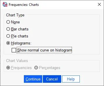
Next, click on the “Charts” button on the right menu.
Frequencies Charts Diagrams Dialog Box

The Diagrams dialog box opens with a selection of several chart types. In our case, we choose Histograms and click Continue.
Ready to Start

The selection of statistics is complete, and now the calculations can be started. To do this, we click OK.
Interpreting the Results
Statistics Table
SPSS displays all results in the output window. In the left column, we see a table of contents, which is particularly useful for maintaining an overview in case of multiple calculations. In the large field, we find the actual calculations, tables, titles, and notes.
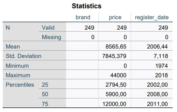
The first ‘Statistics’ table includes several parameters like Mean, Standard Deviation (Std. Deviation), etc. In statistics, the letter N denotes the number of cases studied. SPSS differentiates between Valid and Missing Values. In our case, we examine 249 cars.
The average price of the cars is €8,565.65, and the average registration date is 2006.
Note: The column in the table of contents can be adjusted by clicking and dragging the frame. The contents of the output are not static. We can adjust the headings and add our own remarks.
Tables for Frequencies
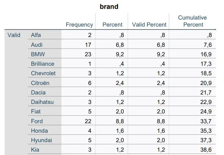
We scroll down to the Frequency Tables. Looking at the ‘Brand’ variable: In the first column, we see the appearing manufacturers, and in the second column are the respective frequencies. Manufacturer Alfa appears twice in the dataset, Audi has 17 cars, and BMW 23. The third column shows the relative frequency in the entire sample as a percentage. In our case, 9.2% of all vehicles are from BMW. In the Cumulative Percent column, the individual percentages in each row are summed up step by step.
Histograms
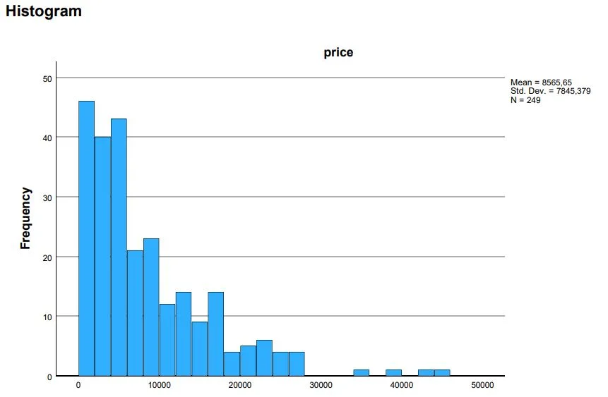
Next, we look at the Histogram for the price. The histogram visualizes the values from the upper frequency table. The X-axis lists the measured values, and the Y-axis shows the frequency for each value.
We observe that the prices are not normally distributed and that a majority of the cars cost less than €10,000.
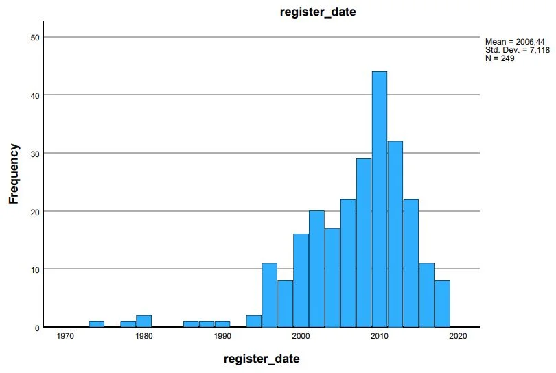
Note: If you want to learn more about normal distribution, check out this tutorial: Checking Normal Distribution – SPSS
What Next?
It depends entirely on your needs. Frequency analyses are essentially an entry point to get an overview or to check specific conditions for more complex calculations. Depending on the research question, several analyses are possible, here are two examples:
- Is there a significant difference between car brands regarding market value? (Analysis of Variance)
- What parameters influence the market price of a used car? (Multiple Regression)

